#피처 데이터 세트 x,레이블 데이터 세트y를 추출
#맨끝이 outcome컬럼으로 레이블 값임. 컬럼 위치-1을 이용해 추출
y=diabetes_data['Outcome']#X=diabetes_data.iloc[:,-1]도 가능함;;
X=diabetes_data.loc[:,(diabetes_data.columns!='Outcome')]#Y=diabetes_data.iloc[:,:-1]
#학습용 피쳐 데이터 셋, 테스트용 피쳐 데이터 셋 , 학습용 타겟 데이터 셋, 테스트용 타겟 데이터 셋
X_train,X_test,y_train,y_test= train_test_split(X,y,test_size=0.2,random_state=156,stratify=y)

# 로지스틱 회귀로 학습,예측 및 평가 수행.
lr_clf = LogisticRegression(solver='liblinear')#solver='liblinear'
lr_clf.fit(X_train, y_train)#학습용 피쳐 데이터 셋, 학습용 타겟 데이터 셋 입력
pred = lr_clf.predict(X_test)#인자는 테스트용으로들어감
pred_proba = lr_clf.predict_proba(X_test)[:, 1]
#비율을 계산,[:, 1]를 입력안하면 0일때의 확률과 1일떄의 확률이 모두 나옴으로 하나로 설정-> 1일떄의 확률만 가져오도록 계싼함

get_clf_eval(y_test , pred, pred_proba)#재현율이 높다고 할 수 없네 그렇다면
#재현율을 높이는 방향으로 진행하자, 그래서 모델의 성능향상 진행
import numpy as np
import pandas as pd
import matplotlib.pyplot as plt
%matplotlib inline

from sklearn.model_selection import train_test_split
from sklearn.metrics import accuracy_score, precision_score, recall_score, roc_auc_score
from sklearn.metrics import f1_score, confusion_matrix, precision_recall_curve, roc_curve
from sklearn.preprocessing import StandardScaler
from sklearn.linear_model import LogisticRegression

import numpy as np
import pandas as pd
import matplotlib.pyplot as plt

#파일불러오기

diabetes_data=pd.read_csv('diabetes.csv')
print(diabetes_data['Outcome'].value_counts())
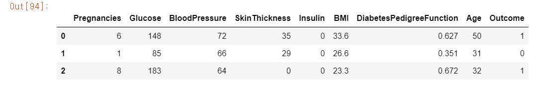
Pregnancies Glucose BloodPressure SkinThickness Insulin BMI DiabetesPedigreeFunction Age Outcome
* Pregnancies: 임신 횟수 *Glucose: 포도당 부하 검사 수치 *BloodPressure: 혈압(mm Hg) *SkinThickness: 팔 삼두근 뒤쪽의 피하지방 측정값(mm) *Insulin: 혈청 인슐린(mu U/ml) *BMI: 체질량지수(체중(kg)/(키(m))^2) *DiabetesPedigreeFunction: 당뇨 내력 가중치 값 *Age: 나이 *Outcome: 클래스 결정 값(0또는 1) **
- 앞 예제에서 사용된 get_cif_eval()과 precision_curve_plot()재로딩
def get_clf_eval(y_test, pred=None, pred_proba=None):
    confusion = confusion_matrix( y_test, pred)
    accuracy = accuracy_score(y_test , pred)
    precision = precision_score(y_test , pred)
    recall = recall_score(y_test , pred)
    f1 = f1_score(y_test,pred)
    # ROC-AUC 추가
    roc_auc = roc_auc_score(y_test, pred_proba)
    print('오차 행렬')
    print(confusion)
    # ROC-AUC print 추가
    print('정확도: {0:.4f}, 정밀도: {1:.4f}, 재현율: {2:.4f},\
          F1: {3:.4f}, AUC:{4:.4f}'.format(accuracy, precision, recall, f1, roc_auc))


   import matplotlib.pyplot as plt
import matplotlib.ticker as ticker
%matplotlib inline

def precision_recall_curve_plot(y_test , pred_proba_c1):
    # threshold ndarray와 이 threshold에 따른 정밀도, 재현율 ndarray 추출.
    precisions, recalls, thresholds = precision_recall_curve( y_test, pred_proba_c1)

    # X축을 threshold값으로, Y축은 정밀도, 재현율 값으로 각각 Plot 수행. 정밀도는 점선으로 표시
    plt.figure(figsize=(8,6))
    threshold_boundary = thresholds.shape[0]#147개가 X축이 됨
    plt.plot(thresholds, precisions[0:threshold_boundary], linestyle='--', label='precision')
    plt.plot(thresholds, recalls[0:threshold_boundary],label='recall')

    # threshold 값 X 축의 Scale을 0.1 단위로 변경
    start, end = plt.xlim()
    plt.xticks(np.round(np.arange(start, end, 0.1),2))

    # x축, y축 label과 legend, 그리고 grid 설정
    plt.xlabel('Threshold value'); plt.ylabel('Precision and Recall value')
    plt.legend(); plt.grid()
    plt.show()
-logistic regression 으로 학습 및 예측 수행
#피처 데이터 세트 x,레이블 데이터 세트y를 추출
#맨끝이 outcome컬럼으로 레이블 값임. 컬럼 위치-1을 이용해 추출
y=diabetes_data['Outcome']#X=diabetes_data.iloc[:,-1]도 가능함;;
X=diabetes_data.loc[:,(diabetes_data.columns!='Outcome')]#Y=diabetes_data.iloc[:,:-1]
#학습용 피쳐 데이터 셋, 테스트용 피쳐 데이터 셋 , 학습용 타겟 데이터 셋, 테스트용 타겟 데이터 셋
X_train,X_test,y_train,y_test= train_test_split(X,y,test_size=0.2,random_state=156,stratify=y)

# 로지스틱 회귀로 학습,예측 및 평가 수행.
lr_clf = LogisticRegression(solver='liblinear')#solver='liblinear'
lr_clf.fit(X_train, y_train)#학습용 피쳐 데이터 셋, 학습용 타겟 데이터 셋 입력
pred = lr_clf.predict(X_test)#인자는 테스트용으로들어감
pred_proba = lr_clf.predict_proba(X_test)[:, 1]
#비율을 계산,[:, 1]를 입력안하면 0일때의 확률과 1일떄의 확률이 모두 나옴으로 하나로 설정-> 1일떄의 확률만 가져오도록 계싼함

get_clf_eval(y_test , pred, pred_proba)#재현율이 높다고 할 수 없네 그렇다면
#재현율을 높이는 방향으로 진행하자, 그래서 모델의 성능향상 진행
### 임곗값의 변경에 따른 정밀도-재현율 변화 곡선을 그림
pred_proba_c1 = lr_clf.predict_proba(X_test)[:, 1]
precision_recall_curve_plot(y_test, pred_proba_c1)
## 각 피처들의 값 4분위 분포 확인
diabetes_data.describe()
#포도당 수치가 0이 된다??Glucose
#혈압이 0이다??BloodPressure
#피하지방이 0이다?ㅋㅋSkinThickness
-Glucose의 분포도를 확인해보자.
import seaborn as sns
sns.distplot(diabetes_data['Glucose'], kde=False)
#0에 값이 존재한다.
0값이 있는 피처들에서 0 값의 데이터 건수와 퍼센트를 계산
# 0값을 검사할 피처명 리스트 객체 설정
zero_features = ['Glucose', 'BloodPressure','SkinThickness','Insulin','BMI']

# 전체 데이터 건수
total_count = diabetes_data['Glucose'].count()

# 피처별로 반복 하면서 데이터 값이 0 인 데이터 건수 추출하고, 퍼센트 계산
for feature in zero_features:
    zero_count = diabetes_data[diabetes_data[feature] == 0][feature].count()
    print('{0} 0 건수는 {1}, 퍼센트는 {2:.2f} %'.format(feature, zero_count, 100*zero_count/total_count))
# zero_reatures 리스트 내부에 저장된 개별 피처들에 대해서 0 값을 평균 값으로 대체
diabetes_data[['Glucose', 'BloodPressure','SkinThickness','Insulin','BMI']]
diabetes_data[zero_features].mean()
#이렇게 한번에 해도 되는구나!

#zero_features 리스트 내부에 저장된 개별 피쳐들에 대해서 0값을 평균 값으로 대체
diabetes_data[zero_features]=diabetes_data[zero_features].replace(0,diabetes_data[zero_features].mean())

# 0값을 검사할 피처명 리스트 객체 설정
zero_features = ['Glucose', 'BloodPressure','SkinThickness','Insulin','BMI']

# 전체 데이터 건수
total_count = diabetes_data['Glucose'].count()

# 피처별로 반복 하면서 데이터 값이 0 인 데이터 건수 추출하고, 퍼센트 계산
for feature in zero_features:
    zero_count = diabetes_data[diabetes_data[feature] == 0][feature].count()
    print('{0} 0 건수는 {1}, 퍼센트는 {2:.2f} %'.format(feature, zero_count, 100*zero_count/total_count))

#이제없어짐!!
#재현율과 정밀도가 함께 좋아지는 정도는 임곗값이 0.48 정도 일 것 같다..
# 임곗값를 0.48로 설정한 Binarizer 생성
binarizer = Binarizer(threshold=0.48)

# 위에서 구한 lr_clf의 predict_proba() 예측 확률 array에서 1에 해당하는 컬럼값을 Binarizer변환.
pred_th_048 = binarizer.fit_transform(pred_proba[:, 1].reshape(-1,1))

get_clf_eval(y_test , pred_th_048, pred_proba[:, 1])